Well-Mixed Greenhouse Gas Cycles🔗

Carbon Cycle🔗

Introduction🔗

The carbon cycle sub-model is adapted from the FREE model (Fiddaman, 1997). While the original FREE structure is based on primary sources that are now somewhat dated, we find that they hold up well against recent data. Calibration experiments against recent data and other models do not provide compelling reasons to adjust the model structure or parameters, though in the future we will likely do so.

Other models in current use include simple carbon cycle representations. Nordhaus’ DICE models, for example, use simple first- and third-order linear models (Nordhaus, 1994, 2000). The first-order model is usefully simple, but does not capture nonlinearities (e.g., sink saturation) or explicitly conserve carbon. The third-order model conserves carbon but is still linear and thus not robust to high emissions scenarios. More importantly for education and decision support, neither model provides a recognizable carbon flow structure, particularly for biomass.

Socolow and Lam (2007) explore a set of simple linear carbon cycle models to characterize possible emissions trajectories, including the effect of procrastination. The spirit of their analysis is similar to ours, except that the models are linear (sensibly, for tractability) and the calibration approach differs. Socolow and Lam calibrate to Green’s function (convolution integral) approximations of the 2x CO₂ response of larger models; this yields a calibration for lower-order variants that emphasizes long-term dynamics. Our calibration is weighted towards recent data, which is truncated, and thus likely emphasizes faster dynamics. Nonlinearities in the C-ROADS carbon uptake mechanisms mean that the 4x CO₂ response will not be strictly double the 2xCO₂ response.

Structure🔗

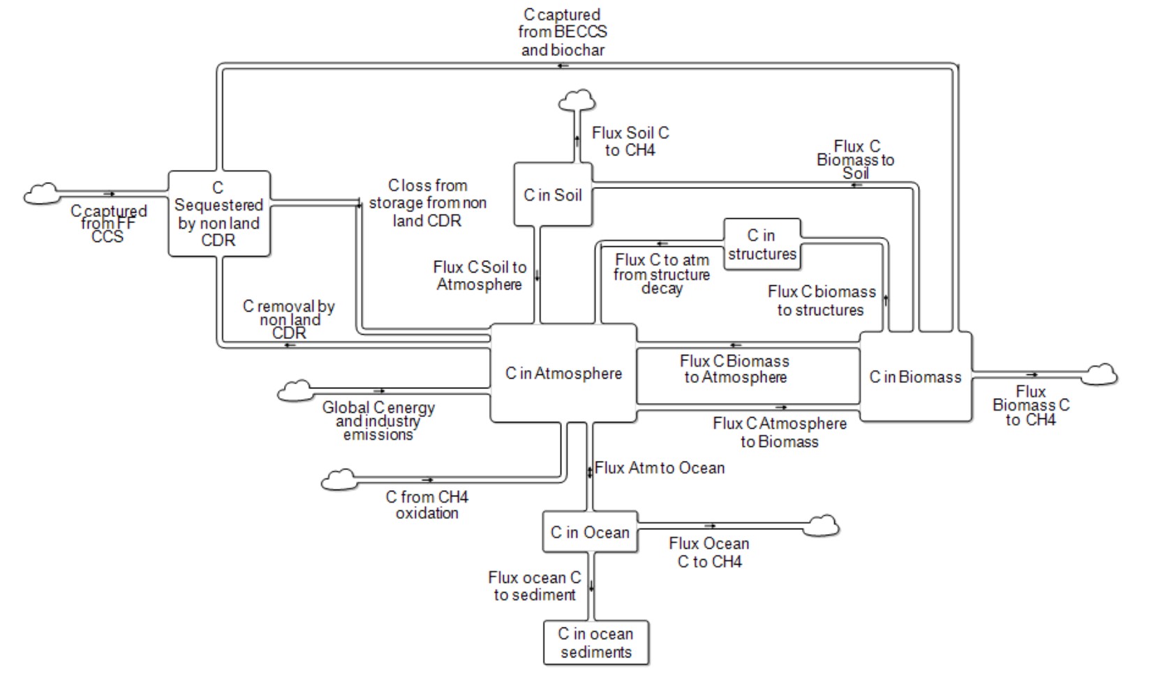
The adapted FREE carbon cycle is an eddy diffusion model with stocks of carbon in the atmosphere, biosphere, mixed ocean layer, and three deep ocean layers. The model couples the atmosphere-mixed ocean layer interactions and net primary production of the Goudriaan and Kettner and IMAGE 1.0 models (Goudriaan and Ketner 1984; Rotmans 1990) with a 5-layer eddy diffusion ocean based on (Oeschger, Siegenthaler et al., 1975) and a 2-box biosphere based on (Goudriaan and Ketner 1984).

The global terrestrial biosphere carbon cycle fluxes and initial biomass and soil stocks are the sum of those by land type as defined in Terrestrial Biosphere Carbon Cycle.

The interaction between the atmosphere and mixed ocean layer involves a shift in chemical equilibria (Goudriaan and Ketner, 1984). CO₂ in the ocean reacts to produce HCO–3 and CO=3. In equilibrium,

$$ C_m = C_{\mathrm{m,0}} \biggl( \frac{C_a}{C_{\mathrm{a,0}}} \biggr) ^ { \frac{1}{\zeta} } $$

C_m = C in mixed ocean layer
C_m,0 = reference C in mixed ocean layer
C_a = C in atmosphere
C_a,0 = reference C in atmosphere
ζ = buffer factor

The atmosphere and mixed ocean adjust to this equilibrium with a time constant of 1 year. The buffer or Revelle factor, ζ, is typically about 10. As a result, the partial pressure of CO₂ in the ocean rises about 10 times faster than the total concentration of carbon (Fung, 1991). This means that the ocean, while it initially contains about 60 times as much carbon as the preindustrial atmosphere, behaves as if it were only 6 times as large.

The buffer factor itself rises with the atmospheric concentration of CO₂ (Goudriaan and Ketner, 1984; Rotmans, 1990) and temperature (Fung, 1991). This means that the ocean’s capacity to absorb CO₂ diminishes as the atmospheric concentration rises. This temperature effect is another of several possible feedback mechanisms between the climate and carbon cycle. The fractional reduction in the solubility of CO₂ in ocean falls with rising temperatures. Likewise for the temperature feedback on C flux to biomass, we assume a linear relationship, likely a good approximation over the typical range for warming by 2100. The sensitivity parameter that governs the strength of the effect on the flux to the biomass also governs the strength of the effect on the flux to the ocean. For both effects, the default sensitivity of 1 yields the average values found in Friedlingstein et al., 2006.

$$ \zeta = \zeta_0 + \delta_b \ln \biggl( \frac{C_a}{C_{\mathrm{a,0}}} \biggr) $$

ζ = buffer factor
ζ₀ = reference buffer factor
δ_b = buffer CO₂ coefficient
C_a = C in atmosphere
C_a,0 = reference C in atmosphere

The deep ocean is represented by a simple eddy-diffusion structure similar to that in the Oeschger model, but with fewer layers (Oeschger, Siegenthaler et al., 1975). Effects of ocean circulation and carbon precipitation, present in more complex models (Goudriaan and Ketner, 1984; Björkstrom, 1986; Rotmans, 1990; Keller and Goldstein, 1995), are neglected. Within the ocean, transport of carbon among ocean layers operates linearly. The flux of carbon between two layers of identical thickness is expressed by:

$$ F_{\mathrm{m,n}} = \frac{ (C_m - C_n) ^ e }{ d^2 } $$

F_m,n = carbon flux from layer m to layer n
C_k = carbon in layer k
e = eddy diffusion coefficient
d = depth of layers

The effective time constant for this interaction varies with d, the thickness of the ocean layers. To account for layer thicknesses that are not identical, the time constant uses the mean thickness of two adjacent layers. The following table summarizes time constants for the interaction between the layers used in C-ROADS, which employs a 100 meter mixed layer, and four deep ocean layers that are 300, 300, 1300, and 1800 meters, sequentially deeper. Simulation experiments show there is no material difference in the atmosphere-ocean flux between the five-layer ocean and more disaggregate structures, including an 11-layer ocean, at least through the model time horizon of 2100.

The carbon cycle also includes removals from carbon dioxide removal (CDR) technologies and any leak or loss rates from storage.

Other greenhouse gases🔗

Other GHGs included in CO₂equivalent emissions🔗

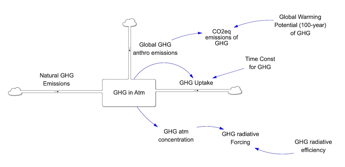
C-ROADS explicitly models other well–mixed greenhouses gases, including methane (CH₄), nitrous oxide (N₂O), and the fluorinated gases (PFCs, SF₆, and HFCs). PFCs are represented as CF₄-equivalents due to the comparably long lifetimes of the various PFC types. HFCs, on the other hand, are represented as an array of the nine primary HFC types, each with its own parameters. The structure of each GHG’s cycle reflects first order dynamics, such that the gas is emitted at a given rate and is taken up from the atmosphere according to its concentration and its time constant. Initialization is based on data from GISS for CH₄, N₂O, and PFCs, and assumed zero for SF₆ and HFCs. The remaining mass in the atmosphere is converted, according to its molecular weight, to the concentration of that gas. The multiplication of each gas concentration by the radiative coefficient of the gas yields its instantaneous radiative forcing (RF). This RF is included in the sum of all RFs to determine the total RF on the system.

For those explicitly modeled GHGs, the CO₂ equivalent emissions of each gas are calculated by multiplying its emissions by its 100-year Global Warming Potential. Time constants, radiative forcing coefficients, and the GWP are taken from the IPCCs Fifth Assessment Report (AR5) Working Group 1 Chapter 8. (Table 8.A.1. Lifetimes, Radiative Efficiencies and Metric Values GWPs relative to CO₂).

For those explicitly modeled GHGs, the CO₂ equivalent emissions of each gas are calculated by multiplying its emissions by its 100-year Global Warming Potential. Time constants, radiative forcing coefficients, and the GWP are taken from the IPCCs Fifth Assessment Report (AR5) Working Group 1 Chapter 8. (Table 8.A.1. Lifetimes, Radiative Efficiencies and Metric Values GWPs relative to CO₂).

In addition to the anthropogenic emissions considered as part of the CO₂ equivalent emissions, CH₄, N₂O, and PFCs also have a natural component. The global natural CH₄ emissions are from the anaerobic respiration of biomass, soil, and oceans. The global natural N₂O emissions are based on MAGICC output, using the remaining emissions in their “zero emissions” scenario. The global natural PFC emissions are calculated by dividing Preindustrial mass of CF₄ equivalents by the time constant for CF₄. Figure 7.2 illustrates the general GHG cycle. The units of each gas are: MtonsCH₄, MtonsN₂O-N, tonsCF₄, tonsSF₆, and tonsHFC for each of the primary HFC types. To calculate the CO₂ equivalent emissions of N₂O, the model first converts the emissions from MtonsN₂O-N/year to Mtons N₂O/year.

CH₄ is unique in that there are additional natural emissions from permafrost and clathrate. The sensitivity of this release defaults to 0.1% per degree Celsius over a threshold, defaulted to 2 Degrees Celsius; the user may change these assumptions.

Montréal Protocol Gases🔗

Rather than explicitly modeling the cycles of the Montreal Protocol (MP) gases, whose emissions are dictated by the MP, En-ROADS uses the calculated RF for historical and projected concentrations, inputted as a data variable.

Cumulative Emissions🔗

C-ROADS calculates the cumulative CO₂ with the initial value taken as the 1990 C-ROADS value starting in 1870. Cumulative emissions are determined through the simulation. The trillionth ton is a marker of cumulative emissions above which a two degree future is far less likely. Budgets are also presented from 2011 and from 2018, based on IPCC thresholds.

Model Structure🔗