En-ROADS Dynamics🔗

As you use En-ROADS, pay attention to when and how much slider adjustments result in departures from the Baseline Scenario. Ask your audience to reflect on why this happened to illuminate thinking about the dynamics of the climate and energy system that En-ROADS simulates.

Most of the dynamics in En-ROADS can be answered by these explanations:

Complex Interactions Between Competing Energy Supplies and Demand🔗

1. Delays and Capital Stock Turnover🔗

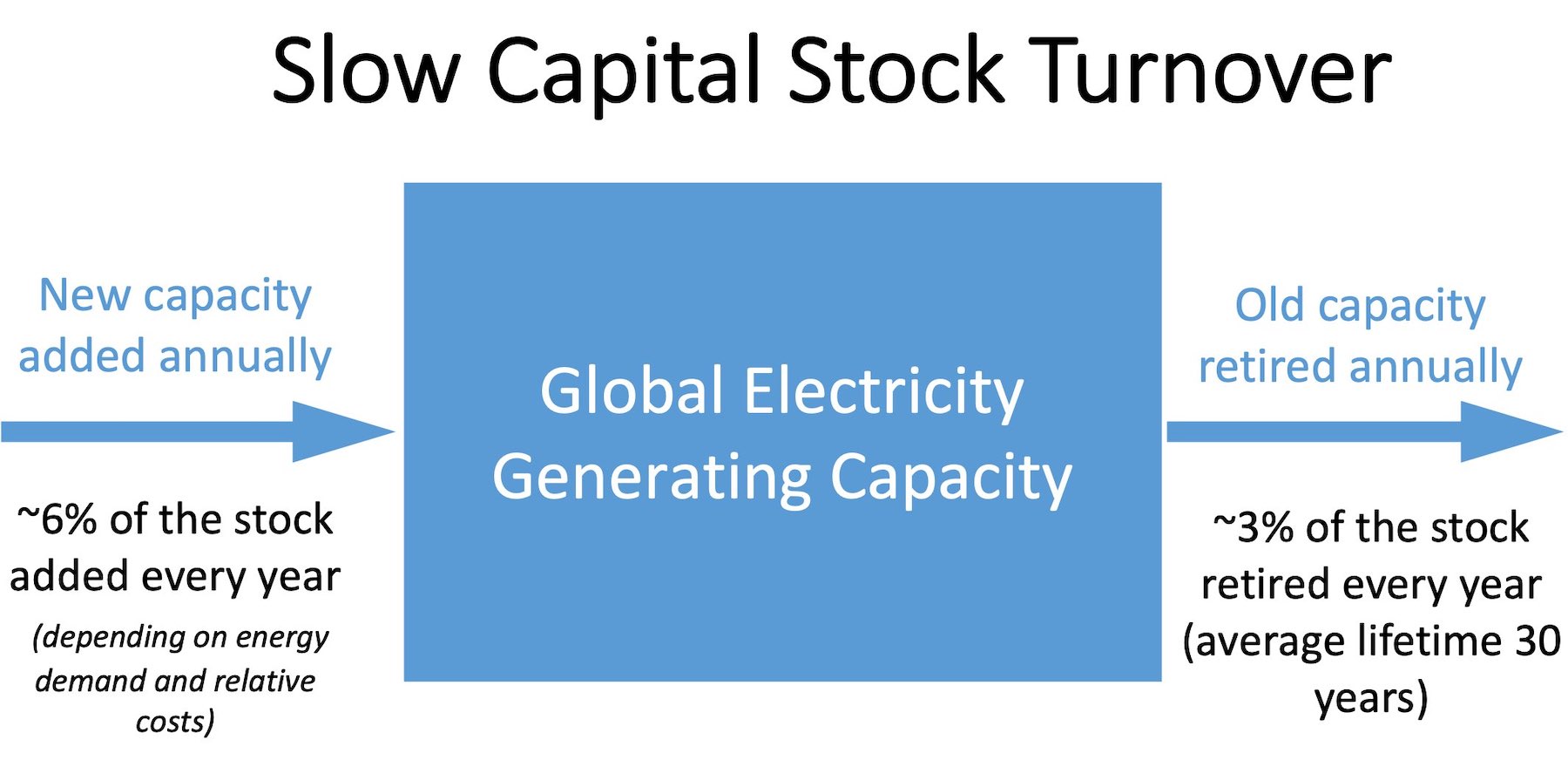
New energy sources (e.g., renewables and new zero-carbon energy sources) take decades (not years) to scale up sufficiently to compete with coal, oil, and gas globally. One of the main sources of these delays is that new energy infrastructure is only built when old infrastructure retires or there is a need to meet increased energy demand.

Only about 6% of all the world’s energy infrastructure changes each year, since infrastructure like coal-fired power plants and oil refineries can be used for 30 or more years. So while new zero-carbon energy sources may make up the majority of the market share of new energy capital, it will take many years for the old capital to turn over and be retired. The climate is only helped when coal, oil, and gas is retired, and in the absence of other interventions, that amount is relatively small — approximately 3% per year.

This addresses questions such as:

• “Why doesn’t subsidizing renewables, nuclear, or a new zero-carbon energy source help avoid more warming?”

This dynamic is also relevant to increasing energy efficiency or electrification. However, energy-using capital, such as vehicles, buildings, and industry, has an average lifetime that is much shorter (10-15 years). One can promote the sale of electric cars immediately, for example, but the average amount of all cars that are electric takes decades to rise to the same level since it takes time for all the old fuel-based cars to be taken off the road.

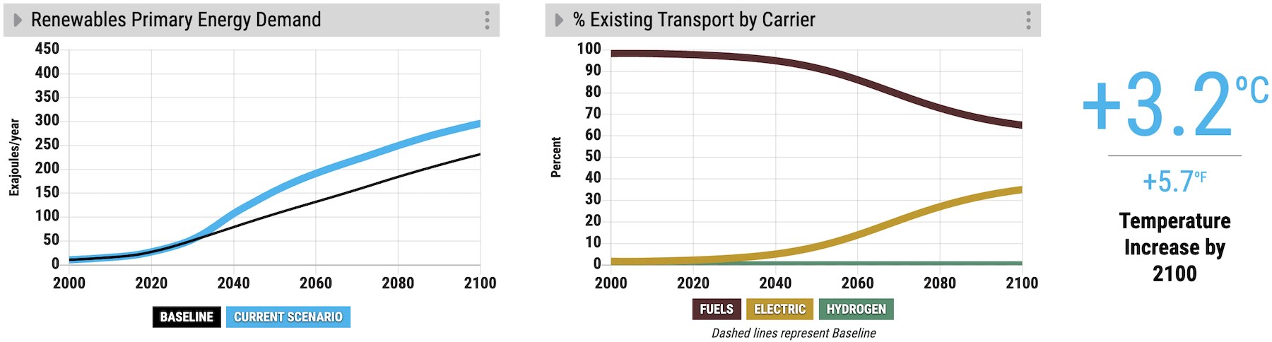
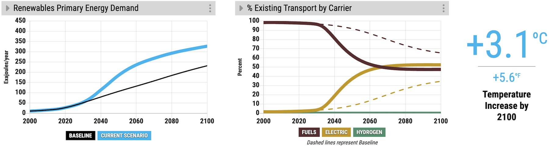
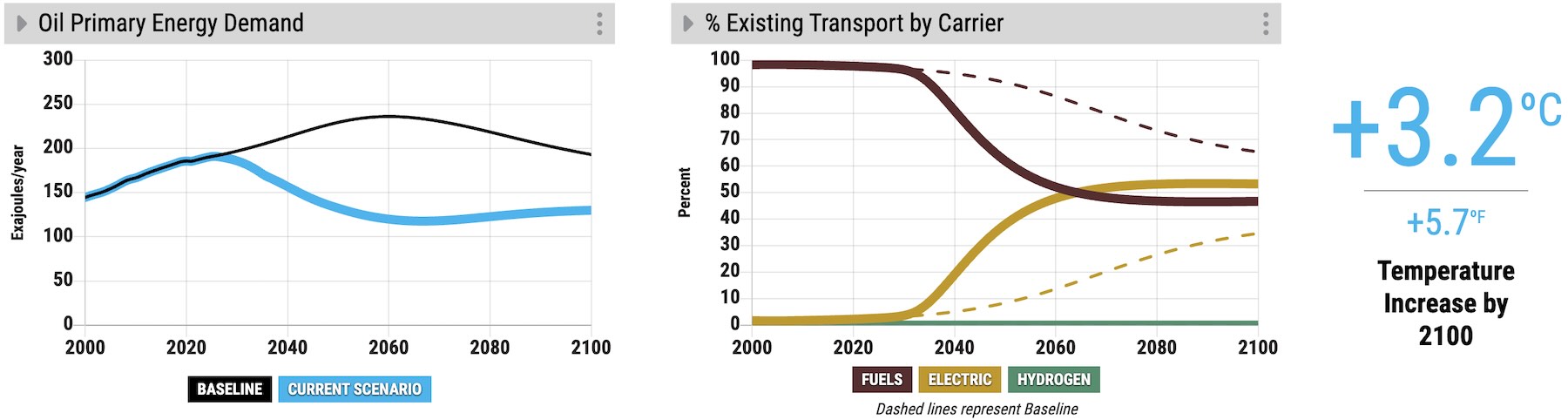
To illustrate this point: Move the Transport Electrification slider to be highly subsidized. Examine the “Electric Share of Total Transport” graph and notice that, even as the amount of electric transport grows, it takes several decades before it can reach over 50% of total transport. Compare this to the graph “Electric Share of Transport Sales” which rises much faster, as sales more immediately reflect the impact of the subsidy.

View this scenario in En-ROADS.

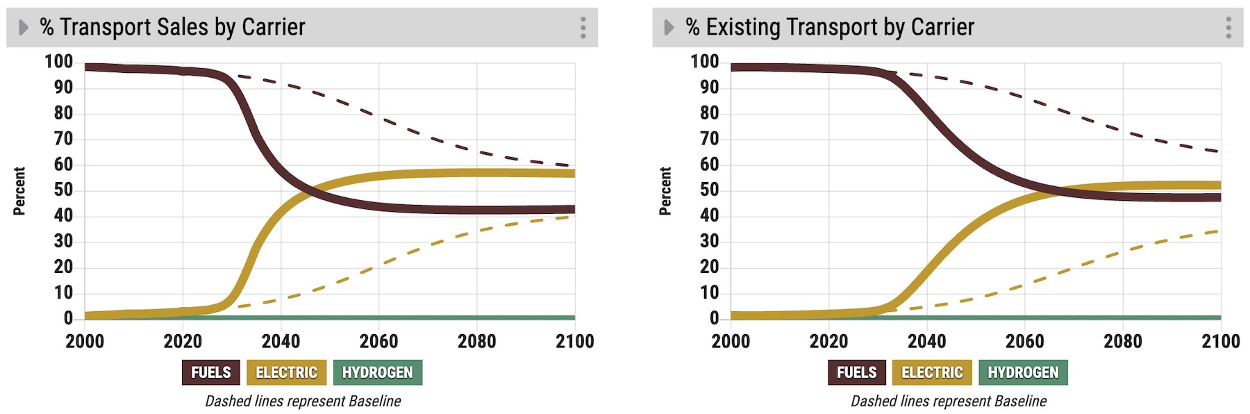
Implications of this dynamic: Policies that merely promote alternatives to fossil fuels take several decades to reduce carbon dioxide emissions — the existing infrastructure takes a long time to retire.

To learn more, view this video on Capital Stock Turnover.

2. Price and Demand Effects🔗

Energy demand falls if energy prices rise, and demand increases if prices fall. People and companies are more likely to take actions to conserve energy (such as turning off lights when they’re not being used), or invest in energy efficiency (such as buying energy-efficient appliances or insulating buildings) when energy prices are high. Policies should be designed to enable people who have a high energy burden (a large proportion of their income going to pay for energy) access to affordable energy and energy efficiency improvements.

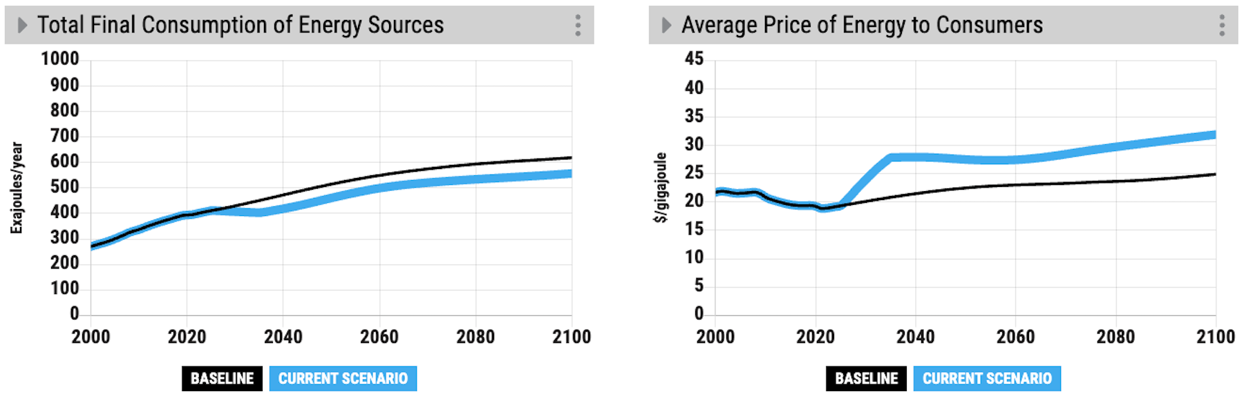
When a high carbon price is set, for example, energy demand falls because energy prices increase. Observe that Total Final Consumption of Energy Sources decreases, while the Average Price of Energy to Consumers increases:

View this scenario in En-ROADS.

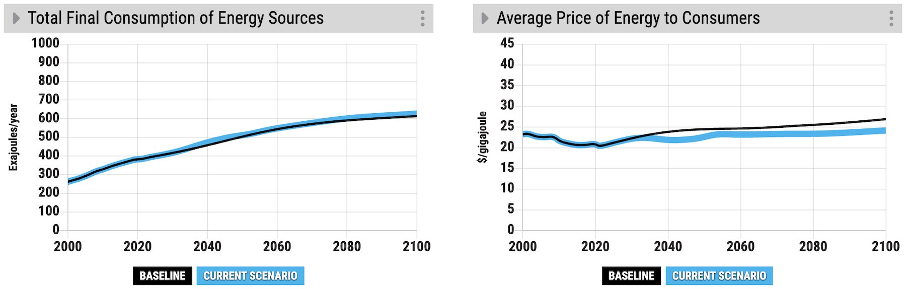
Conversely, energy demand rises when prices fall when a type of energy such as renewables or a new zero-carbon energy source is subsidized or experiences a breakthrough in cost improvement. People and companies are less likely to take actions to conserve energy or invest in energy efficiency when energy prices are low.

Why does the price-demand feedback loop weaken some of the positive effects of subsidizing renewables or other zero-carbon energy sources?

The price-demand feedback loop is one reason why subsidizing renewable and other zero-carbon forms of energy is less effective at reducing CO₂ emissions than you might expect.

Here are the key points to remember about this dynamic:

1. Renewable energy or other low- or zero-carbon forms of energy only help the climate when they replace coal, oil, and gas, preventing those sources from emitting greenhouse gases.
2. When you subsidize renewable or nuclear energy, or you add a breakthrough in a new zero-carbon source of energy that is very cheap, this lowers the overall cost of energy and demand goes up.
3. This increased demand for energy weakens the positive effects of renewables/nuclear/new zero-carbon energy for two reasons:
   • The increased demand for energy is met for the most part by low-carbon energy, but as a result, less low-carbon energy is available to displace fossil fuels.
   • Some of the increased demand may be met by fossil fuels that would otherwise not be needed, which emit greenhouse gases.

If the only sources of energy available did not emit CO₂, then an increase in energy demand would not have an effect on the climate. But in most scenarios, it’s important to disincentivize the burning of coal, oil, and gas in addition to incentivizing low-carbon energy sources.

To learn more, view this video on the Price-Demand Feedback Loop.

3. Competition between Energy Sources: “Crowding Out” and “Squeezing the Balloon”🔗

Many assume that if the world promoted several long-term zero-carbon energy sources such as nuclear, wind, and solar, their contribution to carbon mitigation would be additive. Instead, they actually compete. More of one, less of another.

This addresses questions such as:

• “Why didn’t it help to have a breakthrough in a new zero-carbon energy supply in this renewables-dominated scenario?”

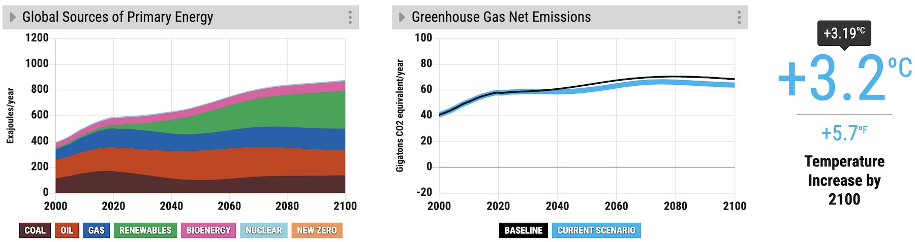
To illustrate this point: See the “Global Sources of Primary Energy” graph in the three scenarios below. In the first graph, we subsidize renewables alone; in the second, there is a breakthrough in a new zero-carbon energy supply; in the third graph, we see both a renewables subsidy and a new zero-carbon breakthrough. Tip: To view the temperature in 2100 to two decimal places, hover over the temperature with your mouse.

In the following scenario, a high Renewables subsidy leads to a 0.10°C (0.2°F) reduction in temperature from the Baseline:

View this scenario in En-ROADS.

A huge breakthrough in New Zero-Carbon leads to a 0.16°C (0.3°F) reduction on its own:

View this scenario in En-ROADS.

When combined, instead of seeing a total 0.26°C (0.5°F) reduction, we only see a 0.23°C (0.4°F) reduction in temperature from the Baseline due to the energy supplies competing with each other for market share:

View this scenario in En-ROADS.

To learn more, view this video on "Crowding Out and Squeezing the Balloon."

4. Complementary Policies: Electrification🔗

Renewables, nuclear, and new zero-carbon energy produce energy in the form of electricity in En-ROADS. Buildings, industry, and transportation need to be able to use electricity in order to use these cleaner sources of energy. Electrification of buildings and industry (for example, by switching to electric heat pumps) and transportation (switching from internal combustion engines to electric vehicles) is therefore essential for changing the energy mix. Notice in En-ROADS how significantly subsidizing Renewables leads to a 0.1 degree Celsius reduction in temperature:

View this scenario in En-ROADS.

And then adding a policy to increase transport electrification lowers the temperature further and boosts demand for renewables:

View this scenario in En-ROADS.

Similarly, in a different scenario, taxing oil is not enough to discourage use of this fuel:

View this scenario in En-ROADS.

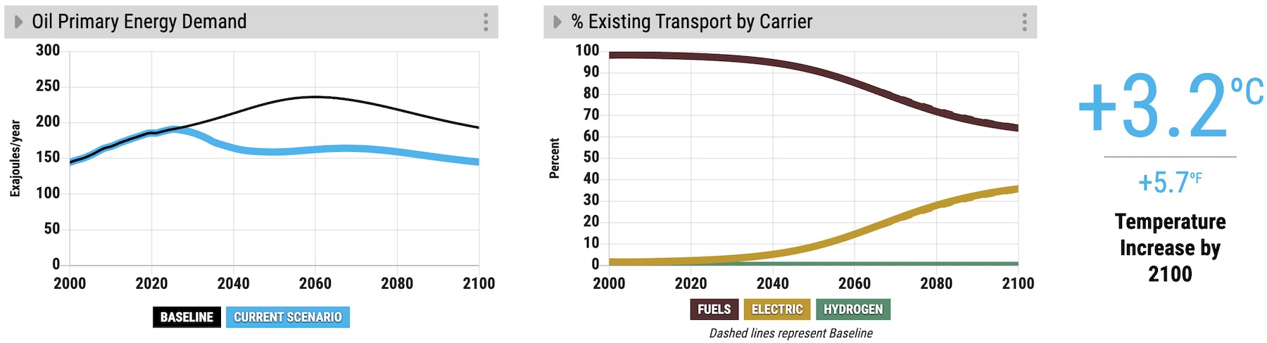
You must also add policies that encourage electrification, which enables things that were dependent on oil to use other sources of energy.

View this scenario in En-ROADS.

5. Economies of Scale and Learning🔗

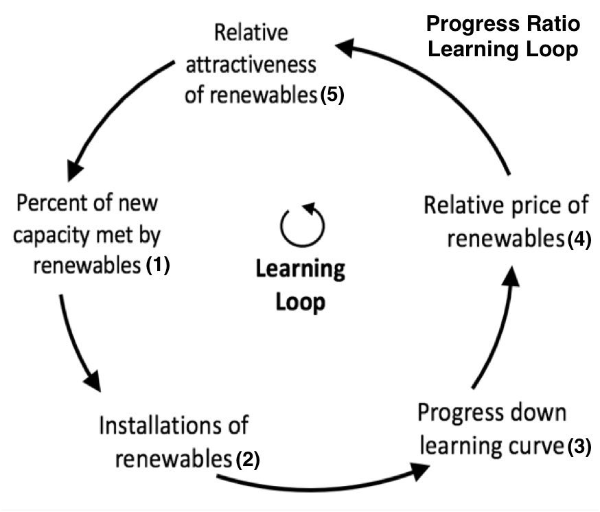
Costs of energy supplies such as renewables fall as cumulative experience is gained through a learning feedback loop, also known as “economies of scale.” Every doubling of cumulative installed capacity of renewables reduces costs by around 20%, creating a reinforcing loop (this is known as the “progress ratio progress ratio: The relative amount of cost reduction per doubling of cumulative production of a technology. In the case of renewable energy, the progress ratio is thought to be 20%, i.e. for every doubling of production, costs decrease by 20%. Costs come down as supply chains, business models, and production industries grow. Also known as the learning effect or learning/experience curve."). In the graphic below, increasing the capacity (1) and installation (2) of new energy sources leads to increased learning (3), a decrease in price (4), increasing the attractiveness of renewables (5) and therefore even greater capacity and installations:

This addresses questions such as:

• “Why should we have hope?”
• “How can we afford a transition to a low-carbon economy?”
• “Aren’t the costs of renewables prohibitive?”

The Economies of Scale dynamic is good news when it comes to renewables. In the past couple decades, the price of renewable energy has dropped significantly and the installation of renewables has grown exponentially. (You can see these trends from 1990 to 2020 in the "Model Comparison - Historical" graphs in En-ROADS).

The progress ratio progress ratio: The relative amount of cost reduction per doubling of cumulative production of a technology. In the case of renewable energy, the progress ratio is thought to be 20%, i.e. for every doubling of production, costs decrease by 20%. Costs come down as supply chains, business models, and production industries grow. Also known as the learning effect or learning/experience curve. for renewables is 0.80, which is quite low compared to other sources of energy such as nuclear and coal (0.98). Remember, a progress ratio of 0.80 means that every doubling of cumulative installed capacity lowers costs 20%. For coal, every doubling of cumulative installed capacity lowers costs just 2%. Coal and other older energy sources have already achieved significant cost reductions due to technological advancements over the past decades.

This also addresses the question “Why is subsidizing renewables helpful?”

Subsidies reduce the cost of renewables, which leads to more installation of renewables, and more cumulative experience (social acceptance, training of installers and engineers, greater availability of factories to make the parts, etc.). The learning loop cycles faster than it would without the subsidies. The same thing would occur without subsidies, but it would be slower. In the meantime, more coal, oil, and gas would be burned and emit greenhouse gases.

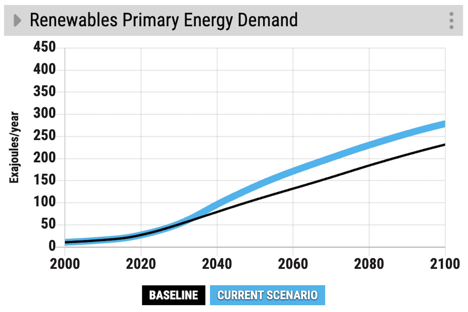
To illustrate this point: Look at the “Renewables Primary Energy Demand” graph in a scenario in which Renewables are subsidized. It increases the exponential growth that is driven and sustained by the reinforcing learning loop figure shown above.

View this scenario in En-ROADS.

To learn more, view this video on Economies of Scale.

6. Economic Damage from Climate Change🔗

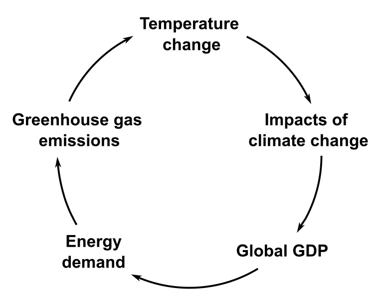
Temperature increase from climate change damages the economy and reduces consumption, slightly reducing some of the future negative effects from climate change. An increase in global temperature is linked to changes in climate patterns—such as more frequent climate disasters, lower crop yields from droughts, etc.—which damage the economy. This reduces GDP growth and global energy consumption. Less consumption produces fewer greenhouse emissions, which results in lower temperature increase. This is a compensating or balancing feedback loop:

This addresses questions such as:

• “Does En-ROADS account for the costs of climate change impacts?”
• “Why do Carbon Removal actions increase Energy Consumption or CO₂ Emissions from Energy?”
• “Why does action on Agricultural Emissions or Waste and Leakage increase Energy Consumption?”

Here are the key points to remember about this dynamic:

1. This dynamic can be turned off with the “Climate change slows economic growth” switch under Simulation > Assumptions > Economy > "Economic impact of climate change." This results in the economy continuing to grow without being affected by climate change, causing more greenhouse gas pollution and more climate change. Note that changing the Assumptions in En-ROADS only affects the Current Scenario, and the economic impact of climate change will continue to be present in the Baseline Scenario. View this scenario in En-ROADS, and turn ON and OFF the “Climate change slows economic growth” switch.

2. Actions (e.g., carbon removal, or reducing Agricultural Emissions or Waste and Leakage) that reduce temperature without affecting energy costs or energy efficiency will still cause energy consumption to increase. The temperature reduction caused by these actions reduces some of the economic impact of climate change, which leads to higher GDP growth and thus more energy consumption and greenhouse gas emissions.
   
   Note that if the only sources of energy available do not emit CO₂, then an increase in energy demand due to higher GDP growth would not have an effect on the climate.

3. Estimates of the effect of climate change on the economy, known as the “damage function,” are varied. The basis of the Baseline Scenario damage function is a study from Burke et al. 2018. If users would like to choose a higher or lower pathway for the damage function, they can select from the functions of other peer-reviewed studies or create their own. Details can be found in this FAQ: Why does En-ROADS include the damage function from Burke et al. (2018) in the Baseline Scenario?

To learn more, read the Explainer on the Economic Impact of Climate Change in En-ROADS.

Drivers of the Baseline Scenario🔗

To gain a deeper understanding of the model’s behaviors, it is important to comprehend what factors drive the Baseline Scenario. Learn more in the En-ROADS Baseline Scenario chapter.

1. Drivers of Growth🔗

A challenge to limiting future warming in this simulation is the powerful growth in global GDP GDP: Gross Domestic Product. The total value (money) of goods produced and services provided in a country during one year. (Gross World Product). This is driven by the Population and Economic Growth sliders. More production and consumption of goods and services requires more energy. While energy efficiency and changes to the fuel mix can help reduce energy emissions, their success is dampened by the growth in GDP. Part of this growth is slowed down by climate change impacts such as lower crop yields, intensified natural disasters, sea level rise, and biodiversity loss. This impact on GDP is known as the “damage function” and slows the increase in consumption and energy demand. However, energy demand and CO₂ emissions from energy are still rising throughout the century, which leads many users to explore different futures for population (for example, by empowering women in developing countries, which could lower population growth) and economic growth measured in GDP per person (for example, by finding ways to meet economic needs without increasing consumption).

This addresses questions such as:

• “We’ve done a lot in energy efficiency and clean energy – why haven’t emissions reduced substantially enough?”

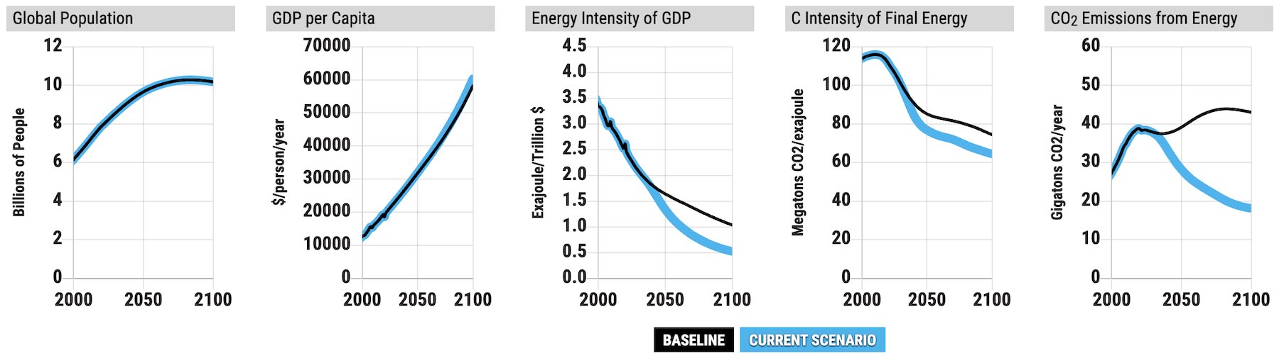
To illustrate this point: See the Kaya Graphs view below for a low-emissions scenario with increased energy efficiency and a transition to low-carbon energy sources. Even though Energy Intensity of GDP improves, and the Carbon Intensity of Energy decreases as well, Global Population and GDP per person continue to grow.

View this scenario in En-ROADS.

To learn more, view this video on the Kaya graphs.

2. Non-CO₂ Emissions Affect Temperature Significantly🔗

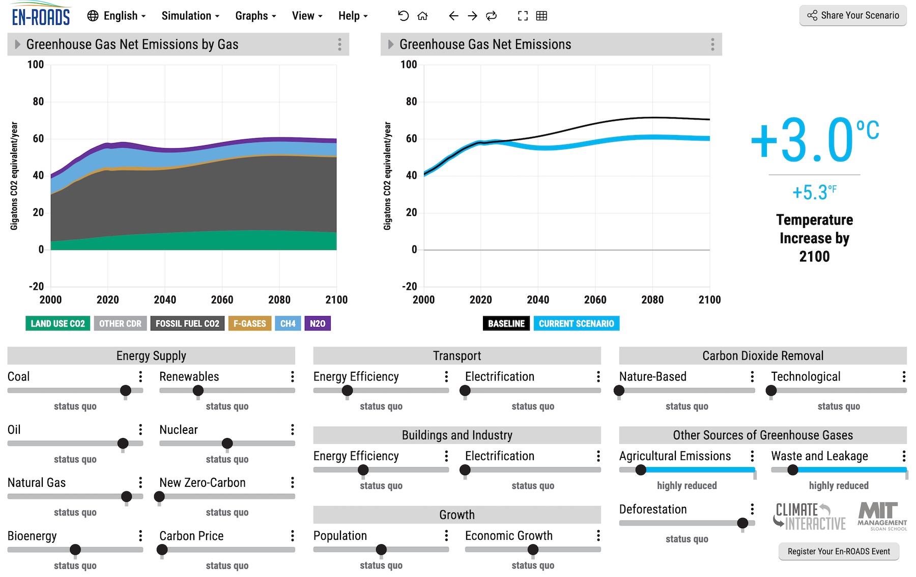
Methane (CH₄), N₂O, and the F-gases are controlled by the Agricultural Emissions and Waste and Leakage sliders. Adjusting these sliders has a large impact on temperature. This implies significant changes in livestock management and consumption, waste management, fertilizer use, and industry. These emissions currently make up around 26% of total greenhouse gas emissions.

This addresses questions such as:

• “We’ve done a lot in energy – why haven’t we solved the climate crisis?”

To illustrate this point: See the “Greenhouse Gas Net Emissions by Gas – Area” and “Greenhouse Gas Net Emissions” graphs and adjust the Agricultural Emissions slider and Waste and Leakage slider. See the scenario below – highly reducing CH₄, N₂O, and F-gas emissions achieves a significant reduction in 2100 temperature.

View this scenario in En-ROADS.

System Dynamics of the Climate🔗

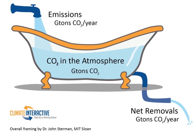
1. Bathtub Dynamics - CO₂ Emissions Must Be Equal to or Lower than CO₂ Removals for Temperature to Stabilize🔗

The metaphor of a bathtub helps explain the dynamics of rising CO₂ concentration in the atmosphere. If more CO₂ enters the atmosphere (like water flowing into a tub) than is removed (like water draining from the tub), then the amount of CO₂ in the atmosphere (the amount of water in the tub) will continue to increase. To flatten CO₂ concentration and therefore temperature, we need to bring CO₂ emissions down to equal removals. If your bathtub is overflowing, you turn off the tap first.

This addresses questions such as:

• “Emissions are stabilized, so why is temperature or CO₂ concentration still going up?”

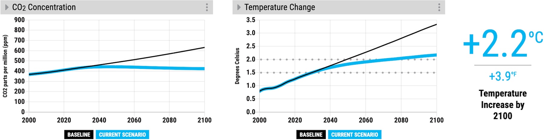
To illustrate this point: See the “CO₂ Emissions and Removals” and “CO₂ Concentration” graphs in a scenario where CO₂ emissions stabilize. Even though CO₂ emissions (in red below) are declining, CO₂ concentration (in blue on the right below) continues to increase because emissions are greater than removals.

View this scenario in En-ROADS.

To learn more, view this video on the Carbon Dioxide Bathtub.

To understand more about stocks, flows, and the bathtub framing below, check out our Climate Leader learning series.

2. Delays in the Climate System🔗

In a scenario where CO₂ concentration stabilizes, global surface temperature continues to increase for a number of years due to heat imbalances between the oceans and atmosphere (this is known as climate inertia). The ocean has absorbed most of the heat trapped by greenhouse gases, but it is slow to reach thermal equilibrium with the atmosphere. Note that the simulation ends in 2100 in En-ROADS, and the time for temperature to stabilize after CO₂ concentration has stabilized may be later than 2100.

View this scenario in En-ROADS.

Please visit support.climateinteractive.org for additional inquiries and support.