Impacts🔗

Drawing on peer-reviewed literature we identified and formulated relationships between En-ROADS output variables and a diverse set of impacts.

Extreme Weather🔗

Deaths from Extreme Heat🔗

As global temperatures rise, deaths from extreme heat are projected to increase. Vicedo-Cabrera et al. (2018) used an exposure-response framework to estimate the relationship between historically observed daily temperature and excess mortality in each study location. The study used 3 Global Climate Models (GCM) to generate daily temperature estimates for all countries included in the study to project temperature-related excess mortality under the RCP8.5 scenario up to 2099, assuming no change in demographics or population vulnerability.

Using the results of Vicedo-Cabrera et al. (2021) Fig. 4(a) we determined the retrospective global estimates for heat-related excess death, as well as those of West Asia and Southern Africa. Assuming the projected global trend of temperature effect on the excess heat-related mortality from Table S3 in Vicedo-Cabrera (2018) applied to each of the two regions, future projections were estimated for West Asia and Southern Africa, overcoming one of the limitations of the 2018 study.

Subsequently, we converted the metric used in the above studies (% of total deaths) to a more commonly used ‘annual deaths per 100,000 people’ using World Bank Open Data for historical population and crude death rates. Finally, we fit exponential lines through the processed data points to get region-by-region as well as global relationships between temperature rise relative to pre-industrial levels and annual heat-related deaths per 100,000 population.

This methodology carries certain caveats. The assumption that the global trends in temperature-related excess mortality apply uniformly to West Asia and Southern Africa may be an underestimate of temperature-related excess mortality risks due to local vulnerabilities. The methodology also inherits sampling biases from the original study, as the data were limited to certain urban populations and geographical areas, as shown in the country list from Table S1 in Vicedo-Cabrera (2018) below. Countries with an * are from Vicedo-Cabrera (2021).

Outdoor Labor Losses from Extreme Heat🔗

As global temperatures rise, outdoor labor losses due to extreme heat are projected to increase. Parsons et al. (2021) illustrated this impact by linking changes in Global Mean Temperature to reductions in work capacity in outdoor heavy labor sectors such as agriculture, forestry, fisheries, and construction.

Using an exposure-response framework based on epidemiological data, the study estimated reduction in work capacity at different hourly Wet Bulb Globe Temperature (WBGT), with productivity losses of <1% at WBGT of 20°C, 10% at 27°C, 50% at ~32.5°C, and 90% losses at ~38°C. Using CMIP6 projections for the 21st century, the study generated estimates for daily WBGT for all countries included in the study (n=163) to aggregate global heavy labor workforce, reported in Figure 3(a) of the article.

We fit an exponential curve to the data from Figure 3(a) having adjusted temperature rise to be relative to pre-industrial levels, and used the global workforce assumptions from the supplementary material of Parsons et al. (2021) to calculate the per worker annual hours/days of labor lost due to rising temperatures, which was converted into 12-hour workdays. By coding this exponential relationship into En-ROADS, we were able to estimate future outdoor heavy labor losses due to temperature rise.

Population Exposed to Tropical Cyclones🔗

As global temperatures rise, more people are projected to be exposed to hurricanes, typhoons, and tropical cyclones as the likelihood of extreme weather events rises.

Studies by Lange et al. (2020) and Geiger et al. (2021) estimated a relationship between temperature rise and the global population at annual risk of exposure to hurricanes, typhoons, or tropical cyclones, defining exposure as encountering hurricane-force winds (≥64 knots wind speed) for at least one minute in a given year.

We digitized and averaged data from these studies to estimate the percentage of the global population annually exposed, using an exponential fit to formulate the relationship between temperature rise and exposure to tropical cyclones in En-ROADS. Multiplying this estimated percentage by total population in En-ROADS gives the results shown in the graph for the population annually exposed to hurricanes, typhoons, or tropical cyclones.

Population Exposed to River Flooding🔗

As global temperatures rise, more people are projected to be exposed to river flooding as the likelihood of extreme weather events rises.

The relationship between temperature rise and the population annually exposed to river floods was derived from Alfieri et al. (2017), Fig. 4(a) and Dottori et al. (2018), Fig. 1(b), defining flood exposure as residing in areas experiencing high-flow events with a return period larger than the value of local flood protections in a given year. These studies estimated vulnerable populations by overlaying population density maps with global flood hazard maps generated by a hydrological model, simulated with projections from 7 climate models.

We normalized the estimates from both studies to constant 2015 populations, allowing us to calculate percentage-based exposure. We fit exponential curves to both sets of results and averaged them to formulate the relationship between temperature rise and exposure to river flooding. Multiplying this estimated percentage by total population in En-ROADS gives the results shown in the graph for the population exposed to river flooding.

Health and Economy🔗

Air Quality–PM2.5🔗

The air quality sector simulates annual global emissions of PM2.5. En-ROADS estimates annual global emissions from three sources: energy generation (electricity), energy generation (non electricity), and other sources (including agriculture and open fires).

Ambient PM2.5 is considered the leading environmental health risk factor globally and is a top 10 risk factor in countries across the economic development spectrum. PM2.5 is fine particulate matter as defined by the mass per cubic meter of air of particles with a diameter of <=2.5 micrometers (µm).

The components of PM2.5 are solid and liquid particles small enough to remain airborne and are defined as two forms:

1. Solids/liquid particles directly emitted to the atmosphere (primary PM).
2. Solids/liquid particles formed from gaseous precursors (secondary PM).

Components of PM2.5 may include (some of) the following:

• Carbons
• Sulfates
• Nitrates
• Chlorides
• Iron
• Calcium
• Other Organics (solid/liquid)

Sources of PM2.5 in En-ROADS – Overview🔗

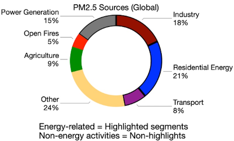
PM2.5 is generated from multiple sources. The chart was from research Global Sources of Fine Particulate Matter: Interpretation of PM2.5 Chemical Composition Observed by SPARTAN using a Global Chemical Transport Model (Weagle et al 2018).

En-ROADS aggregates these sources into the following sources:

1. Energy generation a. Electricity production b. Energy (non electricity) production
2. Non-energy generation a. agriculture, b. open fires, c. other sources.

PM2.5 from Energy Generation🔗

En-ROADS calculates energy generated PM2.5 emissions by applying an emissions factor (EF) (in million metric tons (Mtons) emitted per exajoule (EJ)) for each fuel source to the annual rate of energy produced (in EJ/year).

$$ Emission Rate[Fuel] = EF[Fuel] \times Electricity Production[Fuel] $$

EFs for fuel sources are calculated in several input-output models. En-ROADS applies EFs estimated from analysis by the International Institute for Applied Systems Analysis (IIASA). The EFs for coal, oil, and gas were calculated using the GAINS model (IIASA) to estimate emissions/year from G20 countries/regions and then averaged. Countries included the United States, several EU countries, India (2 regions) and China (3 different regions). The EF for bio was calculated from the RAINS model (IIASA).

Estimates for EFs were not significantly different between electricity and non electricity (which includes industry). En-ROADS applies the same EFs to electricity and non electricity. Users can vary the EF assumption across a range (by source), with a range of 50% to 150% of the base EF (shown in the table below).

PM2.5 from Non Energy Sources🔗

Non-energy sources of PM2.5 are estimated by applying a per capita EF (Mtons/year/billion people) to global population (billion people). The per capita EF is set at the start of the scenario year.

In 2015, non-energy sources of PM2.5 accounted for 35% total PM2.5 emissions. En-ROADs uses that 35% as an estimate of the non-energy contribution to total prior to 2015.

The per capita PM2.5, is calculated in 2015 (Scenario Year) by dividing global non-energy PM2.5 (Mtons/year) by global population in billions (2015). For 2015 and remaining simulated years, non-energy PM2.5 (Mtons/year) is calculated by multiplying global population (billions) by the 2015 emissions factor.

Malaria and Dengue Exposure🔗

As global temperatures rise, exposure to vector-borne diseases is projected to increase. Colón-González et al. (2021) illustrated an example of this impact by linking multiple RCP (Representative Concentration Pathways) scenarios to projections of global population at risk (PAR) of malaria and dengue diseases. Population at risk does not mean catching the disease, rather living in a location where the climatic conditions promote vector transmission for at least one month in a given year.

Using an ensemble of disease models to simulate the transmission of malaria and dengue in the 21st century, the study estimated the effect of warming on the length of disease transmission season (LTS), and the global PAR. The disease models were simulated on a global 0.5 × 0.5 degree latitude–longitude grid using projections of daily temperature, precipitation, and humidity from four global circulation models (GCM) under multiple RCP-SSP combinations.

We estimated the relationship between temperature and the percentage of the global population at risk of malaria, and at risk of dengue, by normalizing the population at risk projections from Figure (A8-Supplementary) and Figure (A9-Supplementary) by their respective SSP scenario population at temperatures corresponding to cutoff timepoints in each RCP scenario (e.g. 2030, 2050, 2100).

We fit a quadratic curve of best fit to that relationship as suggested in Colón-González et al. (2021). We then subtracted the estimated pre-industrial percentage of global population at risk to report the additional population at risk due to warming. We present the additional exposure per 100,000 people, a commonly used metric in Epidemiology reporting.

Crop Yield Decrease from Warming🔗

This graph shows the impact of global temperature increases on crop yields of maize, wheat, rice, and soybean. These four crops provide two-thirds of human caloric intake.

The percentages represent the estimated change in yield due to temperature increase, relative to a reference period of 1981-2010, from Zhao et al. (2017). The strength of this temperature feedback can be changed by the "Effect of temperature on crop yield" slider in the Assumptions. The source study focused on the impact of temperature and did not estimate the impact that changes in rainfall or other climatic effects would have on crop yield.

Decreases in crop yield attributable to rising temperatures vary widely by location. Some areas, such as parts of Central America, have already experienced unprecedented crop losses that have led to famine and migration.

Note: This graph shows only the isolated effect of warming on crop yields. The overall “Crop Yield” graph also accounts for farmers’ adaptations—like improving crop varieties and using new farming practices—that can help offset some of the losses shown here.

Historically global crop yield has been growing to meet food demand (see "Crop Yield" graph for related details).

Crop Nutrient Decrease from CO₂ Concentration🔗

As atmospheric CO₂ levels rise, crops grown under these conditions exhibit reduced concentrations of key nutrients such as zinc, iron, and protein, posing a threat to global nutrition (Myers et al., 2014). Zinc and iron deficiencies are significant public health concerns, with wheat, rice, and maize serving as critical dietary sources of these nutrients.

The relationship between rising atmospheric CO₂ levels and declining crop nutrients was derived from Myers et al. (2014). We digitized the mid-points of impact ranges reported in the paper and calculated the implied percentage change in nutrient content per each ppm increase in CO₂ concentration, given the ambient and elevated CO₂ levels reported in each experiment. This percentage change is built into En-ROADS and connected to CO₂ concentration. The linear relationship which we assume is further supported by Ziska et al. (2016).

While Myers et al. (2014) present nutrient reductions separately, we report average declines in zinc, iron, and protein (relative to 1995 as the baseline year) to ensure comparability with the "Crop Yield Decrease from Warming" graph.

Oceans🔗

Population Exposed to Sea Level Rise🔗

At risk to annual flooding: The number of people living on land that is below annual flood levels. Homes and businesses built on this land may be exposed to flooding every year. Actual flooding may be lower because of sea walls and other flood protection measures.

Living below high tide line: The number of people living on land that is below the high tide line. Homes and businesses below the high tide line would be consistently flooded. Actual flooded land may be lower because of sea walls and other flood protection measures.

In the original study by Kulp & Strauss (2019), future projections of exposed population were based on fixed 2010 population data of coastal communities. To account for population growth to 2100, we scaled this population data based on the global UN population estimates used elsewhere in En-ROADS. However, this method does not account for potential migration or shifts in urban areas, given the uncertainty surrounding where future growth will occur.

Sea level rise and its impacts vary widely by region. Low-lying areas with high population densities and low incomes are the most vulnerable. When land is flooded by sea level rise, people can be forced to move, experience loss of their livelihoods, and face freshwater scarcity. Sea level rise can also worsen gentrification as wealthier residents retreat from ocean-front properties to higher ground inland and displace inland residents already there but who cannot then afford the resulting increase in housing and living costs.

Probability of Ice-free Arctic Summer🔗

An ice-free Arctic summer is when the average September sea ice coverage of the Arctic Ocean is less than one-million km² (approximately 7% of the Arctic Ocean area).

The two year-specific percentages represent the probability that the Arctic will be ice-free in 2050 or 2100, respectively. The final bars represent the probability that the Arctic Ocean will be ice-free at least once prior to 2100, estimated from Sigmond et al. (2018).

An ice-free Arctic Ocean would change the albedo of the Earth, because ocean water is darker than sea ice so it absorbs more of the sun's heat. This means the Earth would warm up faster. The loss of Arctic ice has already impacted animal migration patterns and forced some Indigenous communities to give up traditional livelihoods, like hunting.

Loss in Ocean Life from Warming🔗

Climate change is expected to affect oceans in a variety of ways including changing the average water temperature, dissolved oxygen concentration, pH, and nutrient circulation. Such changes may disrupt marine ecosystems and ocean life, often represented in Earth system models as biomass.

We used data from Tittensor et al. (2021) Figure 1 and Figure 3(b) to estimate the relationship between temperature and the percent loss in ocean biomass, relative to pre-industrial levels, using a linear fit.

We presented three trophic levels to emphasize the phenomenon of trophic amplification, whereby species at a higher level in the food chain are more vulnerable to the effects of climate change due to reduced trophic efficiencies, lengthening of food chains, and higher metabolic costs (Lotze et al., 2019).

Ecosystems and Biodiversity🔗

Arid Land Expansion from Warming🔗

One worrisome land type change is desertification as increased aridity can change an area's capacity to supply ecosystem services or host biodiversity. Increased aridity is often associated with desertification, although recent studies show the relationship is not one-to-one. We used a bias-corrected estimate from the CMIP5 model ensemble from Huang et al. (2016) Figure 2 to link temperature rise to the increased area of arid lands globally. Digitizing the relationship over time under two RCP scenarios, we estimated an exponential relationship between global arid land area and temperature over the 21st century.

Ecosystem Shifts from Warming🔗

A notable projected impact of climate change is the risk of ecosystem shift which was presented in Ostberg et al. (2013) and expanded in Warszawski et al. (2013). Climate change is expected to cause biogeochemical changes in land, which would affect flora and fauna and their interactions, thus impacting ecosystems. The assumption is the larger biogeochemical changes are, the higher the risk of ecosystems being disrupted.

Global land was classified into 16 categories as follows:

Warszawski et al. (2013) used an ensemble of global vegetation models to estimate the percentage of global land area at risk of experiencing ecosystem shifts, from one land type to another, under different temperature scenarios. We digitized the S-shaped relationship from Warszawski et al. (2013) Figure 3 into En-ROADS and linked it to our temperature projections to enable the user to track the impact of different policy scenarios on ecosystems. We converted the percentage to area in million hectares to make it more relevant to En-ROADS users.

Extinction Risk of Endemic Species🔗

As the warming climate disrupts ecosystems, many species confined to a specific region (i.e., endemic species) are expected to be endangered with extinction due to small population sizes, loss of limited habitat, inability to move, and low capacity to adapt.

We digitized data from Manes et al. (2021) Figure 5(b) and fit a logistic curve to estimate the percentage of endemic species at extremely high risk of extinction, as a function of temperature relative to pre-industrial levels. A logistic curve was selected as it was robust for making projections under high warming scenarios, while satisfying a good fit with the data.

The temperature axis for Figure 5(b) was semi-qualitative. We thus made reasonable assumptions on the given temperature ranges, drawing on data from the CMIP6 (SSP) climate projections, to improve the analytical usability of the data from the figure.

Species Losing More than 50% of Climatic Range🔗

These indicators from Warren et al. (2018) estimate the proportion of species in a particular group that is expected to lose more than half of the area that the species can be found (its climatically determined geographic range) due to temperature increase by 2100. This is a measure of global biodiversity loss.

Biodiversity keeps ecosystems healthy, which is an important factor for food production, and clean water and air.

Model Equations🔗