Land Use, Land Use Change, and Forestry🔗

En-ROADS endogenously calculates the land use, land use change, and forestry (LULUCF) net C emissions by explicitly keeping track of each hectare of different land types; the fluxes of changing land types and the use of each land type due to land and energy demands and policies; and the coflow of carbon on the land. The terrestrial biosphere carbon (TBC) cycle accounts for these anthropogenic carbon emissions as well as natural emissions from biomass and soil respiration and releases as CH₄, accounted in the CH₄ cycle, and primary productivity of each land type.

The TBC cycle reflects that cutting down trees releases carbon and stops them from absorbing CO₂ from the atmosphere. While harvesting crops also releases carbon, the approximately annual or faster regrowth time allows the related carbon release to be considered net zero.

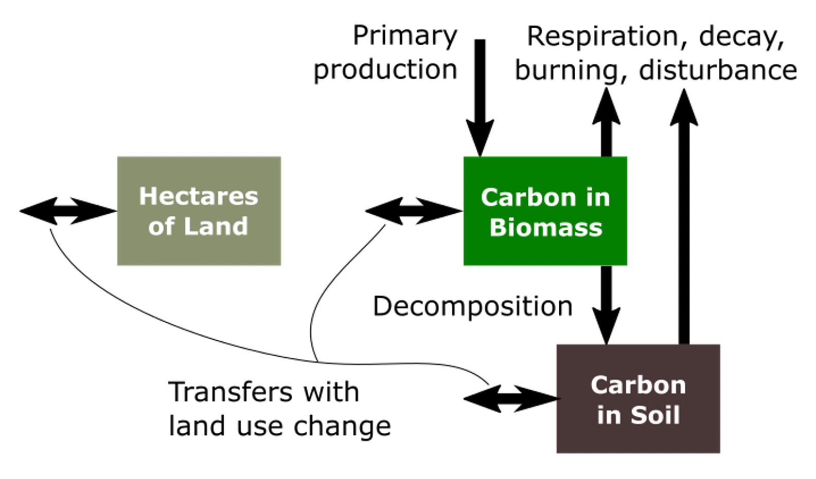
En-ROADS models different kinds of land that can be converted into the others, and the biomass and soil carbon on the land that can accumulate or be released. We have four different land uses: Forest, Agriculture, Other, Tundra; with Forest further divided into three cohorts (Young, 0-50 years; Medium, 50-100 years; and Mature, 100+ years) and whether or not it resulted from afforestation (9 total land uses).

Each type of land has carbon flows:

From the atmosphere to biomass (primary production through photosynthesis)
From biomass to soil (decomposition, etc.)
From soil and biomass to the atmosphere (respiration, decay, burning)
When land use changes, some of the carbon stays on the land and some is released to the atmosphere

Figure 6.1 Land and Carbon Stock and Flow

We cut trees or remove biomass for two reasons: we want the material or we want the land (or both). The material is involved in concepts like bioenergy, wood products, and forest degradation. Needing the land means concepts like deforestation, afforestation, land use change, and agriculture. Those are the policies and scenarios where you can intervene in En-ROADS with each area described below.

Drivers of Deforestation and Degradation🔗

Land that is converted from forest becomes either Farmland (driven by needs of the food system and bioenergy) or Other Land (non-farm deforestation). With six subcategories of forest (NonAF/AF, Young/Medium/Mature), the model assumes that the fraction of deforestation to farmland and to other is proportional to the land area of each to the total forest land.

The primary driver of deforestation has historically been to expand farmland, the need for which is driven by the food system drivers but also by the fraction of farmland expansion that comes from forest. Farmland needs that cannot come from forest comes from Other Land. Farm conversion from other land (mostly grasslands and scrub, but also deserts, barren, urban, etc.) has less effect on the carbon cycle than does deforestation. The fraction of farmland expansion that comes from forest is fixed (at 0.6) in the base case based on historical land use changes.

Non-farm deforestation is exogenous, a simple Baseline scenario based on the LUH data and projections. This reflects forest clearing for development and mining.

The fraction of farmland expansion coming from forests, and the rate of deforestation to other land may be modified by policy inputs. Those inputs come in two modes: from the main Deforestation slider, the input is a percent per year increase or decrease, which results in first order growth or decay relative to the Baseline scenario. In advanced settings, the user can set a year to halt which results in a linear transition to zero in the target year. The policies form reduction rates which are accumulated in a single stock called Relative deforestation which in turn multiplies each component of deforestation rate.

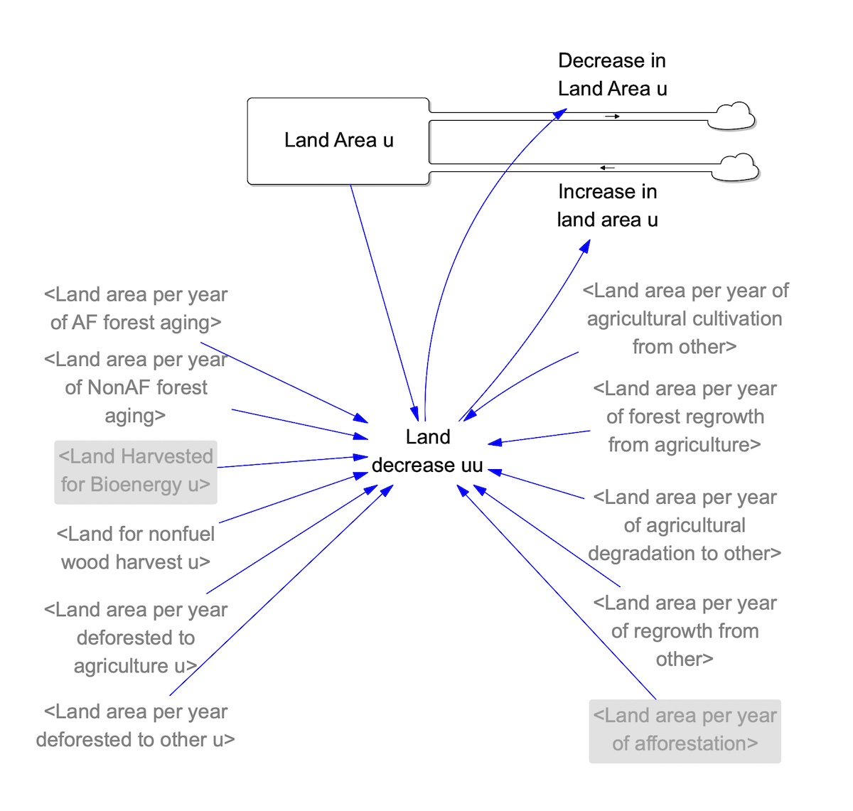
Forests are also harvested and allowed to regrow. The regrowing process can remove carbon from the atmosphere and is therefore often considered carbon-neutral. However, it can take decades to repay the carbon debt incurred with forest harvesting. All forests can be harvested for bioenergy or for wood products. The proportion of total harvest from each forest category is a function of available carbon on each category relative to the total carbon on all forests. A third element that is linked to the main deforestation slider is degradation of mature forest, i.e., forest of average age greater than 100 years. We include it because forest policies often link deforestation and degradation, as in REDD+. Although the terrestrial biosphere structure tracks removal and regrowth of biomass on all forest types, we limit the policies and graphs to degradation of mature forests. Harvest of mature forests is driven by the bioenergy structure, above, along with harvest for non-fuel wood. Non-fuel wood demand (lumber, paper, etc.) is a constant for each region times the population for each region. Structure exists for including a GDP per person effect but the sensitivity is zero.

The policy to directly control degradation is identical to the ones controlling the rate of non-farm deforestation (relative to Baseline) and farm expansion (fraction of expansion from forest), only it affects the fraction of mature forest available for harvest. The main deforestation slider increases or decreases degradation by a percent per year; the advanced view sets a year to halt degradation of mature forests, which also reduces the availability of wood for bioenergy and non-fuel harvest.

There are also command and control-type policies for land conservation; these limits do not address the drivers of deforestation or degradation, but rather prevent those drivers from affecting forest or mature forest. These policies represent the "year to halt" each component.

Food and Agriculture Drivers🔗

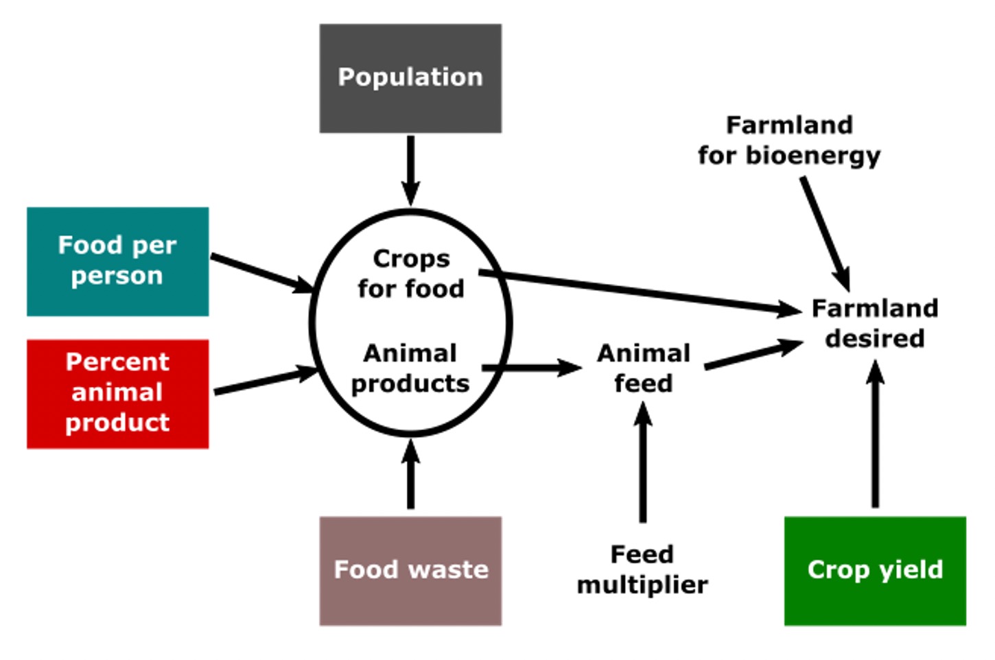
Expanding farmland is a major driver of deforestation and other land use change. We start with the assumption that land will expand to meet food needs. We measure food in kilograms per year, and limit it to two types: crops and animal products. We model a single global food demand and a single global agriculture system. The variables involved in the causality from people to food to land are:

Food per person is modeled as a simple function of GDP per person, fitted to the FAO food balance data, and approaches an upper limit of 900 kg/person/year. There are no user controls for food per person, based on our assumption of meeting food needs.

Percent animal product is the fraction of global diet met by milk, meat, eggs, etc. Consumption of animal product in kg/person/year is a function of global average GDP per person, calibrated to FAO food balance data, from which the fraction is calculated. Under baseline GDP scenarios, it rises from its current value (24%) to a peak of 30% as GDP rises, set by the Food from livestock slider. The current consumption of milk, meat, etc. by region has range from 15% (China and Other Developing B) to over 40% (US), and not strictly arranged by GDP per person; traditional diets play a large part. It is still expected that global animal product consumption will grow over time as countries develop, but En-ROADS allows for users to vary that value between 10% to 40% to be reached in 2100.

Food waste is a single stock that is by default constant at 30%. 30% is the widely quoted but poorly studied value of the amount of food harvested but not consumed, anywhere along the value chain. Anecdotally, it is mostly between farm and market in developing countries, and retail or post-consumer in wealthy countries. If you change the Food waste setting, the new value is reached in 2100 with a linear path.

Food consumption for both crop and animal products is the product of population, food per person, and percent from livestock. Accounting for waste gives production needed to meet that consumption. An additional factor Livestock feed multiplier gives how much plant matter (feed, fodder, grazing vegetation, etc.) it takes to produce each kilogram of animal product. For now that is fixed at 10 kg plant / kg animal product. Farmland desired is then those needs for plant matter divided by yield.

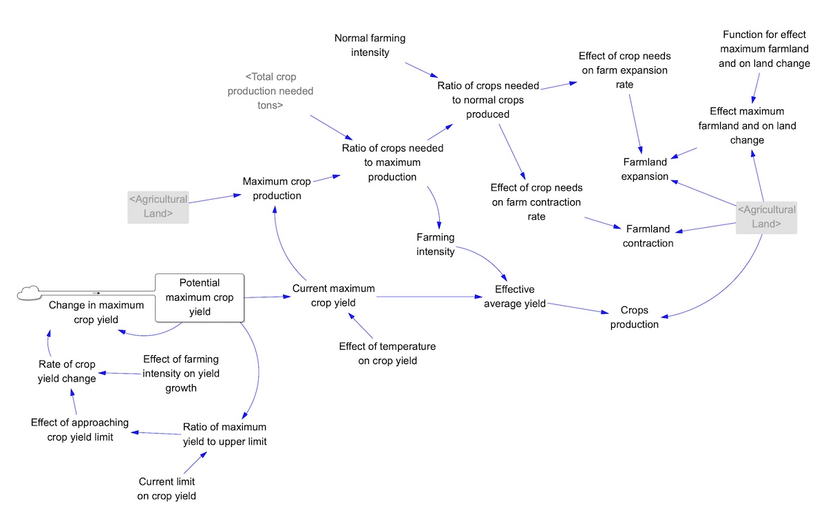
Yield is the global aggregate production of crops, animal feed, pasture vegetation, etc., per year per hectare. The crop yield structure is designed to (1) have Baseline food demand result in land use changes matching LUH projections (2) allow for other yield growth scenarios (3) allow a feedback from temperature to yield (4) have lower yield growth if pressure on food demand is low.

In the data model and supporting files, we find the regression fit to FAO food balance data and use that along with the baseline assumptions to find baseline food demand. The rate of change in implied yield gives a baseline for the potential yield increase over time. The potential is modified up or down by the action of the Crop yield growth slider. The closure of the gap between the potential yield and maximum yield reduces the crop yield growth. The default of the maximum yield set to 2.5 times the 2020 yield implies a comparable growth rate observed since 1960.

The two endogenous reductions to crop yield are low food pressure and high temperature change. Food pressure requiring farming intensity to exceed normal intensity, defaulted to be 0.7, increases the rate of crop yield growth; the converse is true of farming intensity less than normal. It is measured by the ratio of crops needed relative to the crops produced under normal intensity of the farmland, defaulted to 0.7. The integral of crop yield growth is then reduced by the Effect of temperature on crop yield, defaulted to the mean of 4% decrease per degree C, consistent with the Zhao et al (2017) used for the impact table. However, the user may adjust this strength in Assumptions.

Farmland Expansion and Contraction🔗

Farmland expansion occurs when the ratio of crops produced to the crops that could be produced at maximum intensity given the current farmland area exceeds the normal farmland intensity. Conversely, if that ratio is less than the normal farmland intensity, then what is not needed is converted to forest land via natural regrowth, whereas the rest degrades to other land.

Other Land Decreases and Increases🔗

Afforestation policy, i.e. the action depending on the Afforestation slider of En-ROADS, is implemented as the conversion of other land to forest land, since the land identified to be available for afforestation, excludes existing forests and agricultural land and falls into the other land category. Afforestation, as a policy implementation, is formulated based on a user-defined fraction of the full potential of afforestable land, and its delayed conversion to afforested land, which results in the land flux of Land afforestation rate. This flux is then incorporated into the land use change module as a chain of conversions from the other land to young forests and then aging to medium and mature forests. Deforestation from afforested land to farmland and other land affects the efficacy of this policy. The model captures historical regrowth of other land to nonAF young forest. Other land also decreases with farmland expansion, as only a fraction of the expansion comes from forests.