Ocean Systems🔗
Introduction🔗
Ocean systems model the transport of heat, carbon, and alkalinity between ocean layers; and calculate the impacts of sea level rise and ocean acidification. These model sectors overlap and interface with the Carbon Cycle and Climate sectors. We represent a single global ocean with a well-mixed surface layer and four deep ocean layers. Differences across seasons and locations are not included.
The model is adapted from the climate and carbon cycle sectors of the FREE model (Fiddaman, 1997), which was in turn based on the DICE model (Nordhaus 1994) and the work of Schneider and Thompson (1981). The atmosphere-mixed ocean layer interactions and 5-layer eddy diffusion include elements from Goudriaan and Ketner (1984), IMAGE 1.0 (Rotmans 1990), Oeschger et al. (1975), and Large et al. (1994). This formulation is designed to be clear to users, have explicit and conserved material flows, allow for a range of assumptions, and calibration against data sources.
Climate Cycle🔗
Temperature change is calculated for both land and ocean areas as described in the Climate sector. The areas share a common radiative forcing (RF) from greenhouse gases and other factors, but calculate individual temperature changes and feedback cooling from outbound longwave radiation Overall temperature change is an area-weighted average of land and ocean temperatures. Atmosphere over the ocean and the upper layer of the ocean are assumed to be well-mixed in terms of heat content and temperature change, but there is a delay in further heat transfer to the deep ocean layers.
$$ \begin{align} T_\mathrm{surf} &= \frac{Q_\mathrm{surf}}{R_\mathrm{surf}} \\[4pt] T_\mathrm{deep} &= \frac{Q_\mathrm{deep}}{R_\mathrm{deep}} \\[4pt] Q_\mathrm{surf} &= \int (RF(t) - F_\mathrm{out}(t) - F_\mathrm{deep}(t))\,dt + Q_\mathrm{surf}(0) \\[4pt] Q_\mathrm{deep} &= \int F_\mathrm{deep}(t)\,dt + Q_\mathrm{deep}(0) \end{align} $$
T = temperature of surface and deep ocean boxes
Q = heat content of respective boxes
R = heat capacity of respective boxes
RF = radiative forcing
Fout = outgoing radiative flux
Fdeep = heat flux to deep ocean
$$ \begin{align} F_\mathrm{out}(t) &= \lambda \, T_\mathrm{surf} \\[4pt] F_\mathrm{deep}(t) &= \phi \cdot ({Q_\mathrm{surf} - Q_\mathrm{deep}}) \end{align} $$
λ = climate feedback parameter
ϕ = mixing flow rate
The equations for ocean climate are in the same submodel as climate over land, see the listing with the climate equations.
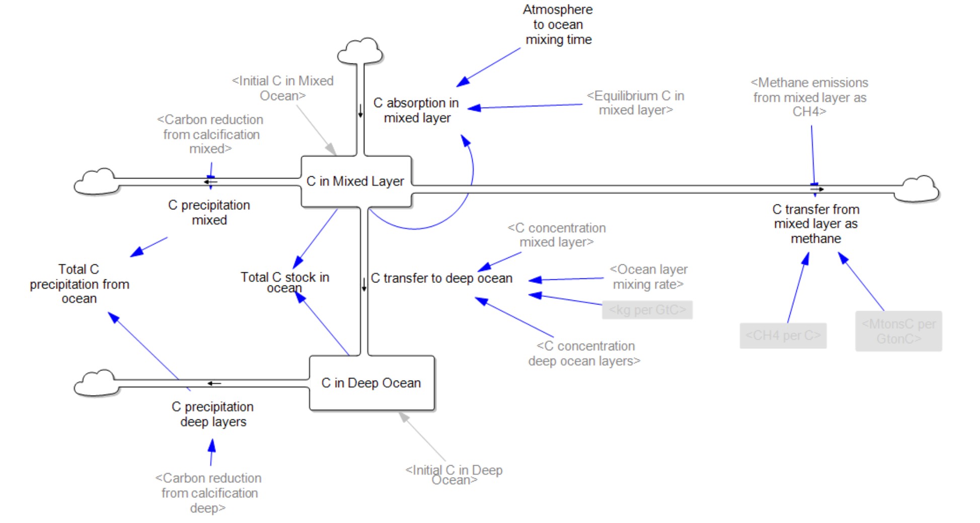
Carbon Cycle🔗
Transfer of carbon between the atmosphere and mixed ocean layer involves a shift in chemical equilibria (Goudriaan and Ketner, 1984). CO2 in the ocean reacts to produce HCO–3 and CO=3, collectively dissolved inorganic carbon (DIC). The equilibrium level of DIC in seawater is a function of CO2 concentration in the atmosphere, alkalinity, temperature, and salinity. Keeping the effect of salinity constant, we approximate the equilibrium value with an empirical function based on chemistry simulations (Gattuso et al. 2026):
$$ DIC_\mathrm{eq} = DIC_\mathrm{ref} \cdot \ (1 - \Delta\ T \cdot \ S_\mathrm{T}) \cdot \biggl( \frac{C_\mathrm{a}}{C_\mathrm{ref}} \biggr) ^ {S_C} \cdot\biggl( \frac{A}{A_\mathrm{ref}} \biggr) ^ {S_A} $$
DIC = Equilibrium and reference DIC in the mixed ocean layer
Δ T = Ocean temperature change from preindustrial
C = Current and reference CO2 concentration in the atmosphere
A = Current and reference alkalinity in the mixed ocean layer
S = Sensitivities of DIC to temperature, CO2, and alkalinity
The atmosphere and mixed ocean adjust to this equilibrium with a time constant of 1 year. The deep ocean is represented by a simple eddy-diffusion structure similar to that in the Oeschger model, but with fewer layers and explicit material flows (Oeschger et al., 1975). Carbon precipitation follows in a fixed ratio from alkalinity calcification, and is a very slow process with a time constant on the order of 100,000 years. Effects of ocean circulation present in more complex models (Goudriaan and Ketner, 1984; Björkstrom, 1986; Rotmans, 1990; Keller and Goldstein, 1995), are neglected. Within the ocean, transport of carbon among ocean layers operates linearly. The flux of carbon between two layers is proportional to the mixing flow rate and the difference in DIC concentrations.
$$ \begin{align} F_\mathrm{m.n}(t) &= \phi \cdot ({C_\mathrm{m} - Q_\mathrm{n}}) \end{align} $$
C = carbon concentration in each layer
ϕ = mixing flow rate
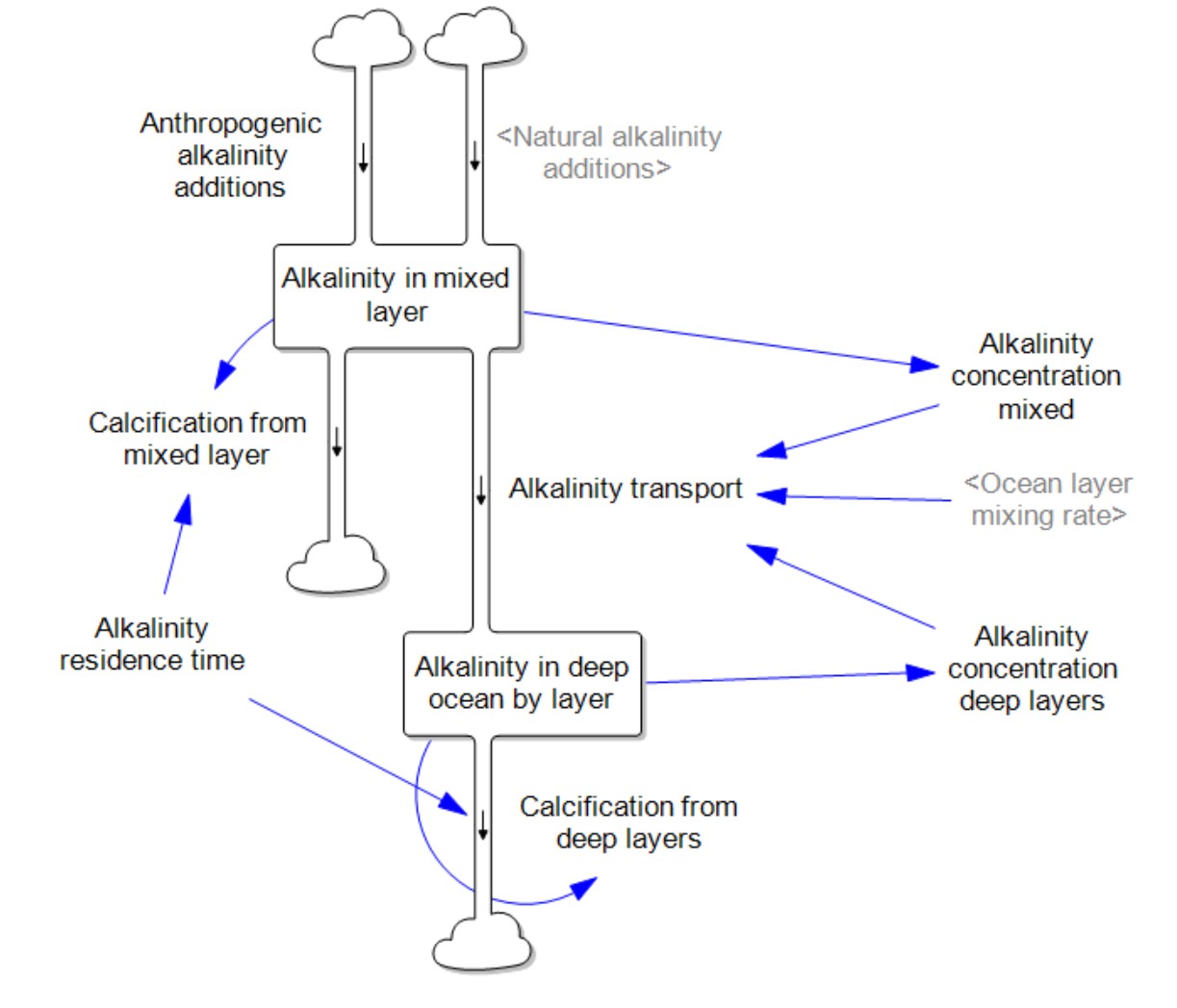
Alkalinity🔗
Alkalinity is the capacity of the oceans to resist changes in pH; it affects the ratio of carbon that exists as dissolved CO2, carbonic acid, carbonates and bicarbonates. Alkalinity is measured in moles of the equivalent chemical effect, or moles per cubic meter (mol/m3) when considering concentration. The molar concentration of alkalinity is an important factor in the calculation of DIC and pH. Alkalinity calcification causes precipitation from all ocean layers into ocean sediments, taking a fixed ratio of carbon with it, over a time constant on the order of 100,000 years. Natural additions of alkalinity from rock weathering are normally in balance with calcification and are assumed constant. Anthropogenic additions of alkalinity as part of ocean alkalinity enhancement (OAE) are calculated in the CDR sector. OAE changes the molar concentration as used in carbon and pH calculations with a first-order delay. Alkalinity transfer between ocean layers is proportional to the difference in molar concentration and the mixing flow rate.
Ocean Acidification🔗
Dissolved CO2 reacts with water to form carbonic acid, which dissociates and shifts the balance of carbonate, bicarbonate, and hydrogen ions, lowering pH and making calcium carbonate less available for shell and skeleton formation (Jiang et al 2019). En-ROADS estimates the average upper ocean pH as an empirical function of dissolved inorganic carbon (DIC), alkalinity, and temperature, based on chemistry simulations (Gattuso et al. 2026). The function is fitted to the Hawai’i Ocean Time series (School of Ocean & Earth Science & Technology 2024) annual average observations of mean seawater pH.
Sea Level Rise🔗
Sea Level Rise (SLR) is modeled by extending the semi-empirical approach proposed by Vermeer and Rahmstorf (2009) in a way to accommodate the water impoundment by artificial reservoirs and to experiment with higher levels of contribution to SLR from ice sheet melting in Antarctica and Greenland than already assumed. The model is estimated from historical data 1900-2021, a period with low levels of warming that therefore may underestimate future sea level rise from the faster-than-historical rates of melt of the Greenland and Antarctic ice sheets. “Contribution to SLR from Ice Melt in Antarctica by 2100” and “Contribution to SLR from Ice Melt in Greenland by 2100” sliders allow users to capture these effects. Sliders are initialized with the mid-range estimates for the contribution of ice sheet melting in Antarctica/Greenland in the IPCC AR6 report.
Model Structure🔗